Scaling Laws For Generative Mixed-Modal Language Models

• Unimodal scaling laws

Modality	α	β
Code	0.37	0.32
Image-Text	0.12	0.11
Image	0.13	0.13
Molecules	0.37	0.26
Speech-Text	0.32	0.24
Speech	0.31	0.24
Text	0.18	0.22

• Unimodal parameters differ widely—Code and Molecules scale “easiest,” Images “hardest”
  • Across 7 modalities (Text, Image, Image-Text, Speech, Speech-Text, Code, Molecules) the fitted α and β exponents range from ~0.11 (Images) to ~0.37 (Code/Molecules).

• Bi-modal scaling law

  • The authors extend Hoffmann-style (a.k.a. “Chinchilla”) scaling to the mixed-modal case by writing the loss for two modalities as the average of the two unimodal scaling laws minus an interaction term C_i,j (benefit) plus small approximation/optimization penalties.
  • $N$ = model size, $D_i$ = dataset on modality $i$
  • A good approximation
    • ${\alpha }_{ij}\approx max({\alpha }_i,{\alpha }_j)$
    • ${\beta }_{ij}\approx max({\beta }_i,{\beta }_j)$
  • 

• $C_{i,j}$ = Maximum synergy: the gap between the best possible joint loss and the average of two separate models

• ${\alpha }_{i,j}$ = how much more model capacity helps with the loss (functional-approx. competition)

• ${\beta }_{i,j}$ = how much more data helps with the loss (optimization competition)

• Modalities compete in the low-compute regime and turn synergistic only after a “competition barrier” is crossed
   • When the interaction term is smaller than the approximation/optimization penalties, each modality drags the other down; the resulting model under-performs two separate unimodal baselines.
   • Once model capacity (N) and data (|D|) are large enough that C_i,j dominates, the same training run becomes strictly better than training two separate models. The paper derives the exact inequality and calls the boundary the competition barrier

  • For Speech + Text, the law forecast a break-even point around a 28 B-parameter model trained on ~45 B tokens.
     • A 30 B parameter run with 50 B tokens indeed beat the two corresponding unimodal baselines, validating the theory.

• Four emergent training phenomena fall directly out of the interaction parameters
   1. Coordinate-ascent behaviour: perplexity for one modality plateaus while another drops, then roles swap—exactly what you expect when modalities “take turns” using limited capacity.
   1.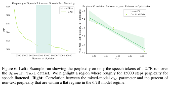  2. The frequency of these plateaus shrinks with larger models and with smaller α_i,j, linking emergence to the functional-approximation term.
   3. Optimal batch size for a mixed run correlates with β_i,j; you can estimate a good batch by summing the unimodal optima and adjusting with β.
   - What the paper found – When the authors swept four global batch sizes (0.5 M → 8 M tokens) for every bi-modal pair, the batch that minimised validation loss almost always satisfied  - $\log \left(\frac{{\text{best‐batch}}_{i,j}}{{\text{best‐batch}}_i+{\text{best‐batch}}_j}\right)\text{∝}{\beta }_{i,j}$  - so higher β_i,j ⇒ a proportionally larger batch is worth paying for .

    - _A larger β means the optimiser needs many fresh examples before each parameter update to overcome that noise. A big batch gives you those examples “in parallel” instead of by adding more steps
    
  

 4. Gradient-spike instability rises roughly with log N / α_i,j, letting the scaling law warn when training will turn unstable. - Large models (N) or small interaction exponents (α_i,j) both push the ratio up and training gets touchier — more spikes, more restarts, lower final quality . - Why it makes sense – α_i,j governs the functional-approximation penalty $\frac{A_{i,j}}{N^{{\alpha }_{i,j}}}$ - When α is small, that penalty falls only slowly as you scale parameters, so the optimiser is forced to chase steep, modality-specific minima. The bigger the log-width of the model (log N) compared with how fast that penalty shrinks (α), the more often gradients “blow up”.