Implementing Flash Attention forward pass

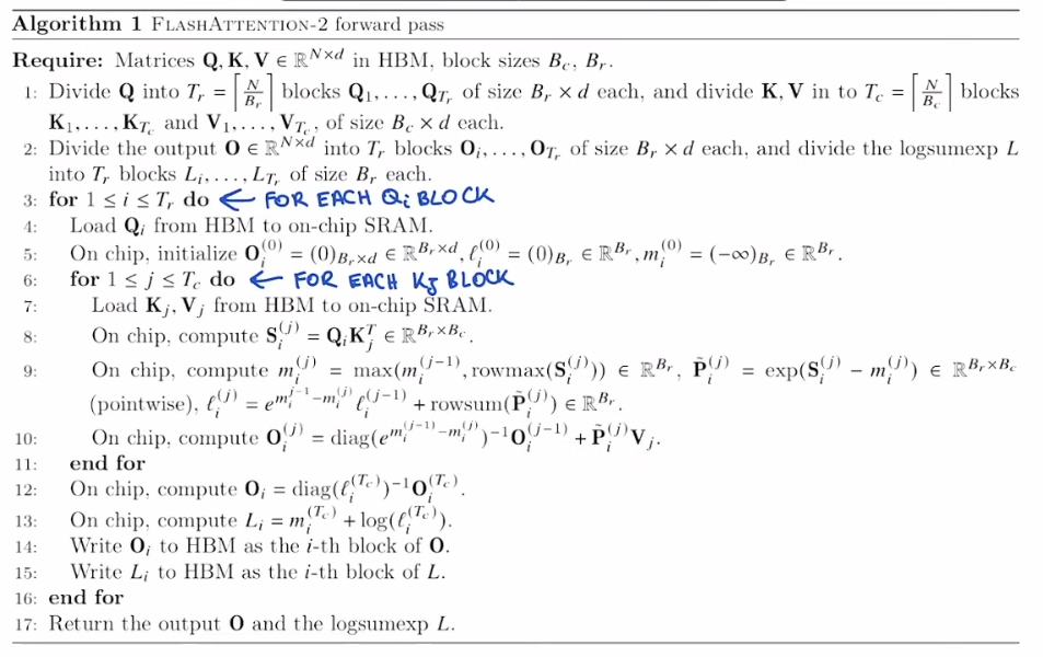
Reminder of the algorithm:

Actual FA2 pseudocode (with more comments on loading between SRAM and HBM)

• This is the code for a single head, within a single sequence within a batch.
• 

What can be parallelized?

• Seeing this code, it’s clear that block of size $B_r\times d$ of the output $O$ is independent of the other blocks.

  • For each of these blocks $O_i$, we will need to load a single query block $Q_i$ , and all the blocks $K_j,V_j$
  • We want to keep the query block $Q_i$ in SRAM for the whole computation

• We can easily parallelize over all the query blocks

• How many programs/kernels do we need to launch then?

  • We will need to launch `batch_size x num_heads x (seq_len // block_size_q)

grid = lambda args: (
triton.cdiv(SEQ_LEN, args["BLOCK_SIZE_Q"]),
BATCH_SIZE* NUM_HEADS,
1
)

Accessing blocks and other optimizations

• Using tl.make_block_ptr and tl.advance abstracts a part of the stride computations, and allows the compiler to optimize memory loads on H100 potentially
• tl.multiple_of(x, N) is a compiler hint: you’re asserting that every element in x is an exact multiple of N (where N is a compile-time constant).
  • Triton doesn’t touch the data—it just records the fact in its IR so that the later optimisation passes and backend code generator can be more aggressive. e.g. pick the aligned variant of HW instructions
  • Practical evidence: in the grouped-GEMM tutorial, adding the hint can make the code 3x faster.

Separating the left-diagonal and diagonal

• Because of block-wise processing, we need to be careful of attending only to the causal K blocks
• We don’t merge the for-loop of the left-diagonal, with the diagonal processing to optimize the pipelining Triton does

Causal Attention Lower Triangular Structure Illustration

=======================================================
In causal attention, each token can only attend to itself and previous tokens.
This creates a lower triangular structure in the attention matrix.
For a sequence of length 8, the attention matrix looks like this:

K₀ K₁ K₂ K₃ K₄ K₅ K₆ K₇

Q₀ ✓ - - - - - - - (Q₀ can only attend to K₀)

Q₁ ✓ ✓ - - - - - - (Q₁ can attend to K₀, K₁)

Q₂ ✓ ✓ ✓ - - - - - (Q₂ can attend to K₀, K₁, K₂)

Q₃ ✓ ✓ ✓ ✓ - - - - (Q₃ can attend to K₀, K₁, K₂, K₃)

Q₄ ✓ ✓ ✓ ✓ ✓ - - - (Q₄ can attend to K₀, K₁, K₂, K₃, K₄)

Q₅ ✓ ✓ ✓ ✓ ✓ ✓ - - (Q₅ can attend to K₀, K₁, K₂, K₃, K₄, K₅)

Q₆ ✓ ✓ ✓ ✓ ✓ ✓ ✓ - (Q₆ can attend to K₀, K₁, K₂, K₃, K₄, K₅, K₆)

Q₇ ✓ ✓ ✓ ✓ ✓ ✓ ✓ ✓ (Q₇ can attend to all K₀-K₇)

  

Where:
- ✓ = allowed attention (masked to 0, not -inf)
- - = masked attention (set to -inf)
- 
Block-wise Processing:
====================
When processing in blocks with different sizes (e.g., BLOCK_SIZE_Q = 2, BLOCK_SIZE_KV = 3):

Block 0 (Q₀,Q₁): Must load 1 block: K₀,K₁,K₂ (left of diagonal)
Block 1 (Q₂,Q₃): Must load 2 blocks: K₀,K₁,K₂,K₃,K₄,K₅ (left of diagonal)
Block 2 (Q₄,Q₅): Must load 2 blocks: K₀,K₁,K₂,K₃,K₄,K₅,K₆ (left of diagonal)
Block 3 (Q₆,Q₇): Must load 3 blocks: K₀,K₁,K₂,K₃,K₄,K₅,K₆,K₇ (left of diagonal)

The diagonal edge case occurs when a K block spans across the causal boundary.

For example, in Block 1 (Q₂,Q₃), the K block [K₃,K₄,K₅] contains:
- K₃: allowed (Q₃ can attend to K₃)
- K₄,K₅: masked (Q₂,Q₃ cannot attend to future tokens)

This requires STAGE 2 processing to handle the mixed masked/unmasked keys within a single K block.

Log-sum-exp “trick”

• For the attention score matrix A= softmax(QK^T) = softmax(X) ## shape (T,T) , each row is defined as $A_{ij}=\frac{exp(x_{ij})-m_i}{{\sum }_{j}exp(x_{ij}-m_i)}$

• Let’s define $l_i={\sum }_{j}exp(x_{ij}-m_i)$

• Assume that in the forward pass, if we store $L_i=m_i+log(l_i)$ for the backward pass (the logsumexp variable)

• Then, in the backward pass, we will recompute $Q{K}^T$, and we can recover $A$ by computing $A_{ij}=exp(x_{ij}-L_i)=\frac{exp(x_{ij}-m_i)}{exp(log(l_i))}=\frac{exp(x_{ij})-m_i}{{\sum }_{j}exp(x_{ij}-m_i)}$